4D Objects By Change - Analysis

This notebook explains how the extraction of 4D Objects By Change (Anders et al., 2020) is run in py4dgeo. For details about the algorithm, we refer to the articles by Anders et al. (2020; 2021).

import py4dgeo

The necessary data for the analysis is stored in an analysis file. There is a dedicated notebook on creating these analysis files. In this notebook, we assume that the file already exists and contains a space-time array with corresponding metadata. You can pass an absolute path to the analysis class or have py4dgeo locate files for relative paths:

analysis = py4dgeo.SpatiotemporalAnalysis("synthetic.zip")

Downloading data from 'https://github.com/3dgeo-heidelberg/py4dgeo-test-data/releases/download/2023-10-20/data.tar.gz' to file '/home/docs/.cache/py4dgeo/d42a93663dec119ee5f65d759a36cde2-data.tar.gz'.
Untarring contents of '/home/docs/.cache/py4dgeo/d42a93663dec119ee5f65d759a36cde2-data.tar.gz' to '/home/docs/.cache/py4dgeo/.'

If needed, the data can be retrieved from the analysis object. Note that this is a lazy operation, meaning that only explicitly requesting such data will trigger the retrieval from disk into memory:

analysis.distances

array([[0.00000000e+00, 2.58459742e-07, 5.09761587e-07, ...,
        0.00000000e+00, 0.00000000e+00, 0.00000000e+00],
       [0.00000000e+00, 2.58459742e-07, 5.09761587e-07, ...,
        0.00000000e+00, 0.00000000e+00, 0.00000000e+00],
       [0.00000000e+00, 2.58459742e-07, 5.09761587e-07, ...,
        0.00000000e+00, 0.00000000e+00, 0.00000000e+00],
       ...,
       [0.00000000e+00, 2.58459742e-07, 5.09761587e-07, ...,
        0.00000000e+00, 0.00000000e+00, 0.00000000e+00],
       [0.00000000e+00, 2.58459742e-07, 5.09761587e-07, ...,
        0.00000000e+00, 0.00000000e+00, 0.00000000e+00],
       [0.00000000e+00, 2.58459742e-07, 5.09761587e-07, ...,
        0.00000000e+00, 0.00000000e+00, 0.00000000e+00]])

In case (part of) the analysis was run before, in this case we do not want to reuse it. We remove previous results via invalidate_results(). By default, all results are invalidated but we may adjust this to keeping the objects or seeds by setting seeds=False or objects=False.

analysis.invalidate_results(seeds=True, objects=True)

[2024-05-14 13:00:18][INFO] Removing intermediate results from the analysis file /home/docs/.cache/py4dgeo/./synthetic.zip

Next, we will construct an algorithm object. You can do so by simply instatiating the RegionGrowingAlgorithm:

algo = py4dgeo.RegionGrowingAlgorithm(
    neighborhood_radius=2.0,
    seed_subsampling=30,
    window_width=6,
    minperiod=3,
    height_threshold=0.05,
)

The neighborhood_radius parameter for this algorithm is of paramount importance: At each core point, a radius search with this radius is performed to determine which other core points are considered to be local neighbors during region growing. This allows us to perform region growing on a fully unstructured set of core points. The seed_subsampling parameter is used to speed up the generation of seed candidates by only investigating every n-th core point (here n=30) for changes in its timeseries. This is only done to improve the usability of this notebook - for real, full analysis you should omit that parameter (using its default of 1).

Further parameters can be set for the change point detection in the time series (cf. Anders et al., 2020). The window_width defines the width of the sliding temporal window that moves along the signal and determines the discrepancy between the first and the second half of the window (i.e. subsequent time series segments). Change point detection is performed using a C++ reimplementation of the Python library ruptures (Truong et al., 2018). The parameter minperiod controls the minimum period of a detected change feature to be considered as seed candidate. The height_threshold (default: 0.0) specifies the required magnitude of a dectected change (i.e. unsigned difference between magnitude at start epoch and peak magnitude).

Next, we execute the algorithm on our analysis object:

objects = algo.run(analysis)

[2024-05-14 13:00:18][INFO] Restoring epoch from file '/tmp/tmp7g7ixq0z/corepoints.zip'
[2024-05-14 13:00:18][INFO] Starting: Find seed candidates in time series
[2024-05-14 13:00:19][INFO] Finished in 0.1754s: Find seed candidates in time series
[2024-05-14 13:00:19][INFO] Starting: Sort seed candidates by priority
[2024-05-14 13:00:19][INFO] Finished in 0.1373s: Sort seed candidates by priority
[2024-05-14 13:00:19][INFO] Starting: Performing region growing on seed candidate 1/70
[2024-05-14 13:00:19][INFO] Finished in 0.1492s: Performing region growing on seed candidate 1/70
[2024-05-14 13:00:19][INFO] Starting: Performing region growing on seed candidate 35/70
[2024-05-14 13:00:19][INFO] Finished in 0.0855s: Performing region growing on seed candidate 35/70
[2024-05-14 13:00:19][INFO] Starting: Performing region growing on seed candidate 59/70
[2024-05-14 13:00:19][INFO] Finished in 0.1118s: Performing region growing on seed candidate 59/70

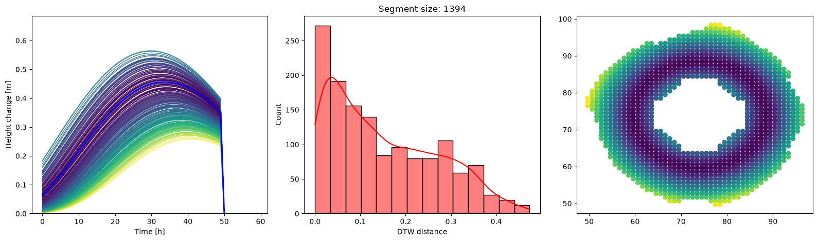
The algorithm returns a list of 4D objects-by-change (segments in the space time domain):

print(f"The segmentation extracted {len(objects)} 4D objects-by-change.")

The segmentation extracted 3 4D objects-by-change.

We can plot single objects interactively:

objects[1].plot()

We can check the timespan and location of the seed by accessing the information stored in the object seed properties:

# Seed coordinate
seed_coord = analysis.corepoints.cloud[objects[1].seed.index]
print(f"Coordinate of seed (XY): {seed_coord[0]:.1f}, {seed_coord[1]:.1f}")

# Seed start and end epoch
print(f"Start epoch: {objects[1].seed.start_epoch}")
print(f"End epoch: {objects[1].seed.end_epoch}")

Coordinate of seed (XY): 66.0, 90.0
Start epoch: 35
End epoch: 71

In this synthetic example there is no reference epoch set. If it were available, we could derive the timestamp of the start and end epochs via the timestamp of the reference epoch in analysis.reference_epoch.timespamp and the temporal offset using the start and end epoch id on analysis.timedeltas.

Note: Similarly to how the M3C2 class can be customized by subclassing from it, it is possible to create subclasses of RegionGrowingAlgorithm to customize some aspects of the region growing algorithm (not covered in detail in this notebook).

References

• Anders, K., Winiwarter, L., Lindenbergh, R., Williams, J. G., Vos, S. E., & Höfle, B. (2020). 4D objects-by-change: Spatiotemporal segmentation of geomorphic surface change from LiDAR time series. ISPRS Journal of Photogrammetry and Remote Sensing, 159, pp. 352-363. doi: 10.1016/j.isprsjprs.2019.11.025.

• Anders, K., Winiwarter, L., Mara, H., Lindenbergh, R., Vos, S. E., & Höfle, B. (2021). Fully automatic spatiotemporal segmentation of 3D LiDAR time series for the extraction of natural surface changes. ISPRS Journal of Photogrammetry and Remote Sensing, 173, pp. 297-308. doi: 10.1016/j.isprsjprs.2021.01.015.

• Truong, C., Oudre, L., Vayatis, N. (2018): ruptures: Change point detection in python. arXiv preprint: abs/1801.00826.