Basic nearest neighbor/C2C algorithm

This notebook demonstrates a basic standard cloud-to-cloud (C2C) distance workflow in py4dgeo.

Implemented by

Ronald Tabernig (@tabernig)

First, import the required packages and helpers:

import py4dgeo
import numpy as np
import pooch

Numba is not installed.
Use `pip install numba` to install it to enable faster computations in Vapc.
You can run py4dgeo.Vapc without Numba, but it may be slower.

Load a small pair of demo point clouds from the same test data used in the other tutorials:

# Set up pooch to download data from Zenodo
p = pooch.Pooch(base_url="doi:10.5281/zenodo.18432391/", path=pooch.os_cache("py4dgeo"))
p.load_registry_from_doi()

try:
    # Download and extract the dataset
    p.fetch("trier_sim.zip", processor=pooch.Unzip(members=["trier_sim"]))

    # Define path to the extracted data
    data_path = p.path / "trier_sim.zip.unzip"
    print(f"Data path: {data_path}")

    before_rockfall_file = (
        data_path / "trier_sim_epoch_0.laz"
    )  # Synthetic data of terrain before a simulated rockfall at Trier study site
    after_rockfall_file = (
        data_path / "trier_sim_epoch_1.laz"
    )  # Synthetic data of terrain after a simulated rockfall at Trier study site

    epoch0, epoch1 = py4dgeo.read_from_las(
        before_rockfall_file,
        after_rockfall_file,
        additional_dimensions={"intensity": "intensity"},
    )


except Exception as e:
    print(f"Failed to download or extract data: {e}")

Extracting 'trier_sim' from '/home/docs/.cache/py4dgeo/trier_sim.zip' to '/home/docs/.cache/py4dgeo/trier_sim.zip.unzip'

Data path: /home/docs/.cache/py4dgeo/trier_sim.zip.unzip
[2026-06-12 12:51:32][INFO] Reading point cloud from file '/home/docs/.cache/py4dgeo/trier_sim.zip.unzip/trier_sim_epoch_0.laz'
[2026-06-12 12:51:32][INFO] Reading point cloud from file '/home/docs/.cache/py4dgeo/trier_sim.zip.unzip/trier_sim_epoch_1.laz'

epoch0 = py4dgeo.epoch.read_from_las( data_path / “trier_sim_epoch_0.laz” ) epoch1 = py4dgeo.epoch.read_from_las( data_path / “trier_sim_epoch_1.laz” )

Instantiate the minimal C2C method and run it on a small corepoint subset:

corepoints = epoch0.cloud[::25]

c2c = py4dgeo.C2C(
    epochs=(epoch0, epoch1),
    corepoints=corepoints,
    max_distance=3.0,
)

distances = c2c.run()

[2026-06-12 12:51:33][INFO] Building KDTree structure with leaf parameter 10

You can optionally enforce mutual matches using correspondence_filter="mutual_nearest_neighbors". Non-mutual matches are kept in place and set to np.nan.

c2c_mnn = py4dgeo.C2C(
    epochs=(epoch0, epoch1),
    corepoints=corepoints,
    max_distance=3.0,
    correspondence_filter="mutual_nearest_neighbors",
)

distances_mnn = c2c_mnn.run()

The next cell allows us to save the C2C results to a LAS file for downstream analysis and visualization.

outputfilepath = "c2c_results.las"

out_vp = py4dgeo.Vapc(epoch=py4dgeo.Epoch(cloud=corepoints), voxel_size=0.1)
out_vp.out = {"c2c_distance": distances, "c2c_distance_mnn": distances_mnn}
out_vp.save_as_las(outputfilepath)

Calling save_as_las
Adding extra dimension 'c2c_distance' of type float64
Adding extra dimension 'c2c_distance_mnn' of type float64
Function 'save_as_las' executed in 0.0279 seconds

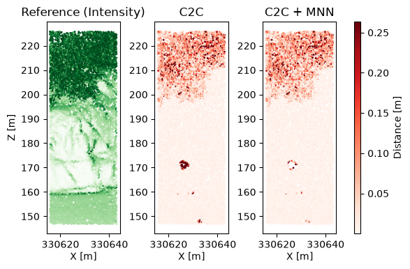
Finally, we generate a 2D preview figure in X–Z view with equal axis spacing: a grayscale intensity reference of the study site (left) and shared-scale C2C and C2C+MNN distance maps (middle/right).

import matplotlib.pyplot as plt
import numpy as np

x = corepoints[:, 0]
z = corepoints[:, 2]
intensities_at_corepoints = epoch0.additional_dimensions["intensity"][
    ::25
]  # Used to color the left reference panel

m0 = ~np.isnan(distances)
m1 = ~np.isnan(distances_mnn)
all_vals = np.concatenate([distances[m0], distances_mnn[m1]])
pmax = 99.0
vmin = np.nanmin(all_vals)
vmax = np.nanpercentile(all_vals, pmax)

i0, i1 = np.nanpercentile(intensities_at_corepoints, [2, 98])

xr = np.ptp(x)
zr = np.ptp(z)
ratio = xr / zr if zr > 0 else 1.0
panel_h = 4.0
panel_w = np.clip(panel_h * ratio, 1.0, 10.0)

fig = plt.figure(figsize=(3 * panel_w + 1.0, panel_h))
gs = fig.add_gridspec(1, 4, width_ratios=[1, 1, 1, 0.06], wspace=0.015)
ax_ref = fig.add_subplot(gs[0, 0])
ax0 = fig.add_subplot(gs[0, 1], sharex=ax_ref, sharey=ax_ref)
ax1 = fig.add_subplot(gs[0, 2], sharex=ax_ref, sharey=ax_ref)
cax = fig.add_subplot(gs[0, 3])

ax_ref.scatter(
    x, z, c=intensities_at_corepoints, s=1, cmap="Greens_r", vmin=i0, vmax=i1
)
ax_ref.set_title("Reference (Intensity)")
ax_ref.set_xlabel("X [m]", labelpad=2)
ax_ref.set_ylabel("Z [m]")

sc0 = ax0.scatter(x[m0], z[m0], c=distances[m0], s=1, cmap="Reds", vmin=vmin, vmax=vmax)
ax0.set_title("C2C")
ax0.set_xlabel("X [m]", labelpad=2)

sc1 = ax1.scatter(
    x[m1], z[m1], c=distances_mnn[m1], s=1, cmap="Reds", vmin=vmin, vmax=vmax
)
ax1.set_title("C2C + MNN")
ax1.set_xlabel("X [m]", labelpad=2)

for a in (ax_ref, ax0, ax1):
    a.set_aspect("equal", adjustable="box")
    a.ticklabel_format(style="plain", axis="x", useOffset=False)

fig.colorbar(sc1, cax=cax, label="Distance [m]")
fig.subplots_adjust(bottom=0.14, top=0.90, left=0.06, right=0.98)
plt.show()